An introduction of parameterization#

What is a parameterization#

Curves can be described algebraically. For example, $y=x^2+3x+2$ is a polynomial which looks like this.

This is an equation where the curve is expressed in terms of x and y, with rational coefficients. However, you can also express this curve as a parameter expression, where you assign a value to the parameter $t$.

The simplest substitution is:

$x=t$

$y=t^2+3t+2$

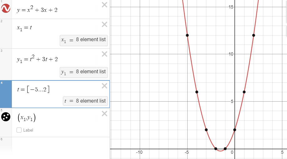
The parameterization matches the algebraic curve

Note, that we have substituted t for x and f(t) for f(x). When we set t equal to the integer range -5 to 2, we see a symmetrical curve which matches the algebraic curve. This is just a different way of thinking about the same shape. In Physics, in the context of motion, the t usually represents time.

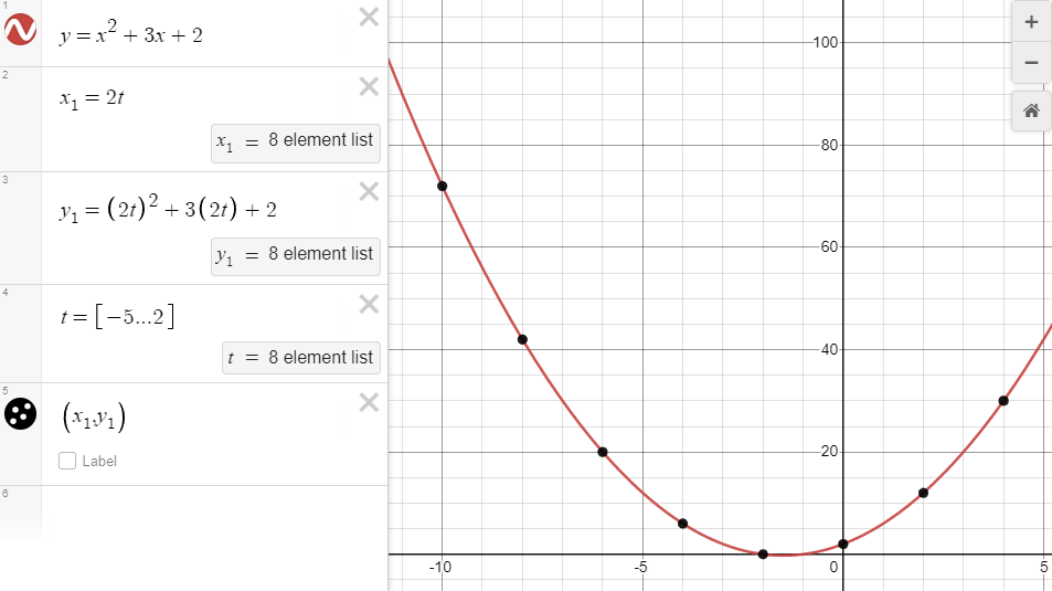
But we don't need to replace x with t. There are actually an infinite number of parametrizations we could use. For instance, we could substitute 2t for x.

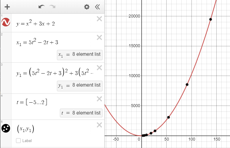
The same curve is matched by the parameter x=2t, but the points lie in different places along the same curve. Note: the points are no longer symmetrical in the range of integers -2 to 5.

You could even use a completely different polynomial for t, and you still end up with points along the same curve. For this example, let's set $x=5t^2-2t+3$

The same curve is matched by the parameter $x=5t^2-2t+3$, but notice that the points are on a much higher scale, and are all positive values. Nevertheless, the points remain of the same algebraic curve.

Parameterization of a circle#

The algebraic equation for a unit circle is $x^2+y^2=1$.

We can substitute t for $\theta$ and use the cosine of the angle as a substitution for x.

$x^2+y^2=1$

$x=\cos t$

$(\cos t)^2+y^2=1$

$y=\sqrt{1-(\cos t)^2}$

If you plot x and y with a t parameter ranging from $0$ to $2\pi$ you will see a semicircle drawn out to $t=\pi$ and then the coordinates will bounce back, retracing the semicircle back to the origin. This is because we haven't accounted for the fact that the actual value of y is $y=\sqrt{1-(\cos t)^2}$ and $y=-\sqrt{1-(\cos t)^2}$

Our trig identities help here. We know the Pythagorean identity: $\sin^2 \theta+\cos^2 \theta=1$ Desmos visualization of Pythagorean identity

So, we can substitute in this way:

$x^2+y^2=1$

$x=\cos t$

$(\cos t)^2+y^2=1$

$\cos^2 t+\sin^2 t=1$

$\therefore y^2=\sin^2t$

$y=\sin t$

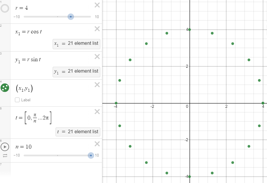
When x=cos t and y=sin t, and when t equals the range from $0$ to $2\pi$ in intervals of $\frac{\pi}{n}$, we find that we have points tracing out the unit circle. This can be scaled to a circle with any radius by replacing $x^2+y^2=1$ with the more general $x^2+y^2=r^2$ For example:

$x^2+y^2=r^2,r=4$

$x^2+y^2=16$

$x=4 \cos t$

$y=4 \sin t$

The parameterization of a circle scales with radius

This parameterization is valid, but is only as precise as the number you round off to when taking the trigonometric functions. What if you needed a rational parameterization instead?

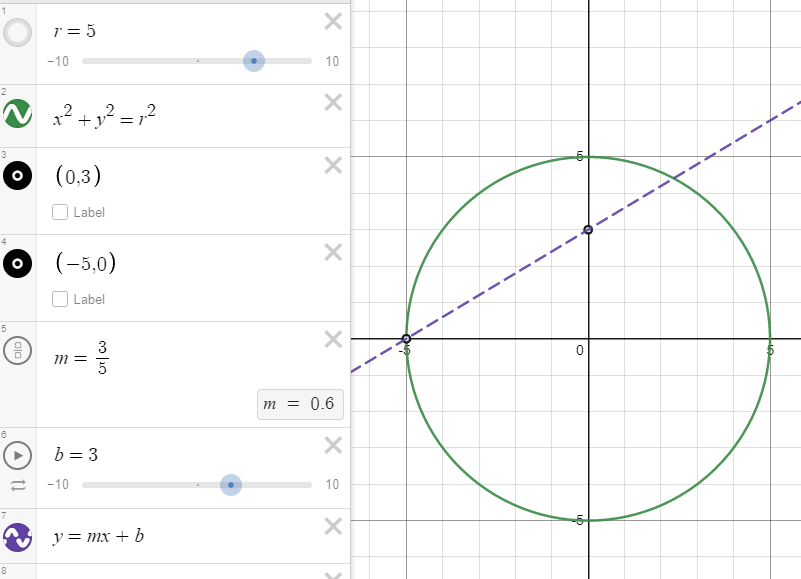
(1) Plot our circle algebraically. Let's say we want to parameterize $x^2+y^2=25$.

(2) Choose a value for t on the y-axis. Let's choose t as the point (0,3).

(3) Select an arbitrary rational point on the circle. Let's choose (-5,0)

(4) Find the equation for the line between (-5,0) and (0,3).

$y=mx+b$

$m=\frac{3}{5}$

$b=y-mx$

$b=3-m(0)$

$b=3$

$y=\frac{3}{5}x+3$

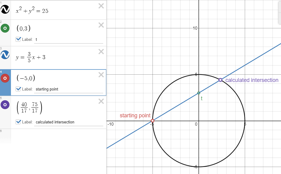
A line passing through the circle at rational point (-5,0) and through the parameter t at point (0,3). The second intersection of the line with the circle must also be rational.

Next we solve for the other point where the line intersects the circle. We are looking at this specific case to make sure the second intersection can be expressed rationally, but then we will find and use a more general form for any value of t.

$y=\frac{3}{5}x+3$

$x^2+y^2=25$

$x^2+y^2-25=0$

$x^2+(\frac{3x}{5}+3)^2-25=0$

$(\frac{3x}{5}+3)(\frac{3x}{5}+3)$

$\frac{9x^2}{25}+\frac{9x}{5}+\frac{9x}{5}+9$

$\frac{9x^2}{25}+\frac{18x}{5}+9$

$x^2+\frac{9x^2}{25}+\frac{18x}{5}+9-25=0$

$\frac{25x^2}{25}+\frac{9x^2}{25}+\frac{18x}{5}+9-25=0$

$\frac{34x^2}{25}+\frac{18x}{5}-16=0$

$\frac{2}{25}\cdot (17x^2+45x-200)=0$

$17x^2+45x-200=0$

$x^2+\frac{45x}{17}-\frac{200}{17}=0$

$x^2+\frac{45x}{17}=\frac{200}{17}$

$(\frac{45}{17})^2=\frac{2025}{1156}$

$(\frac{45}{17})^2+\frac{2025}{1156}=\frac{200}{17}+\frac{2025}{1156}$

$(\frac{45}{17})^2+\frac{2025}{1156}=\frac{15625}{1156}$

$(x+\frac{45}{34})^2=\frac{15625}{1156}$

$x+\frac{45}{34}=\sqrt{\frac{15625}{1156}}$

$x+\frac{45}{34}=\frac{125}{34}$

$x=\frac{125}{34}-\frac{45}{34}=\frac{40}{17}$

$x=-\frac{125}{34}-\frac{45}{34}=-5$

The solution of $x=-5$ we already know, because we began with point (-5,0), however we now also know a rational expression which represents the x component of the second circle intersection with the line at $x=\frac{40}{17}$. Plugging that into our original equation gives us

$y=\frac{3}{5}x+3$

$y=\frac{3}{5}(\frac{40}{17})+3=\frac{75}{17}$

therefore, our second intersection is at $(\frac{40}{17},\frac{75}{17})$ precisely. Both x and y are expressed as rational numbers - an advantage over the approximated trig functions we used earlier.

If the starting point is a rational number, so is the calculated point. We could therefore vary t as a parameter to define rational points on the circle.

To use this rational-to-rational parameterization for any case of t, we need to generalize the equation with the unit circle, point P and parameter t. We will start from point (-1,0) on the unit circle.

$x^2+y^2=1$

$(-1,0)\rightarrow(0,t)$

$m=\frac{t-0}{0+1}=t$

$b=t$

$y=tx+t$

$x^2+(tx+t)^2=1$

$x^2+(tx+t)^2-1=0$

$(tx+t)(tx+t)=(tx)^2+t^2x+t^2x+t^2=(tx)^2+2t^2x+t^2$

$x^2+(tx)^2+2t^2x+t^2-1=0$

$x=[-1] \land [\frac{1-t^2}{t^2+1}]$

In this case, the -1 is known and the x coordinate of point P is $\frac{1-t^2}{t^2+1}$. Substituting this value in the original line equation $y=tx+t$ yields:

$y=tx+t$

$y=t(\frac{1-t^2}{t^2+1})+t$

$y=\frac{2t}{t^2+1}$

Therefore, you may find any Point P on the unit circle for any value of t with

$P=(\frac{1-t^2}{t^2+1},\frac{2t}{t^2+1})$

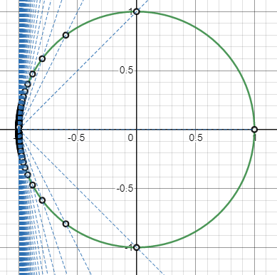
Let's test this out in Desmos with animated values for t = -2 to 2. Notice that even though the values for t go outside the unit circle, the general calculation still finds the second point of intersection, thus defining the circle in rational coordinates.

There is a disadvantage with this kind of parameterization for some scenarios. The calculated points tend to cluster around the starting point for high values of t. You trade the radial symmetry of trigonometric parameterization for the precision of rational coordinates on the circle.

Rational parameterization of a circle from t=-100 to t=100 favoring points near the starting point. Lacks radial symmetry.

Parameterizing other conics#

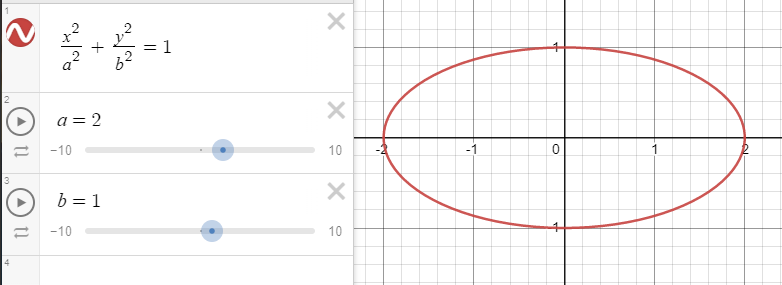
The circle is a simple case, but the same parameterization technique works for other conic sections as well. For instance, let's create an ellipse, centered at the origin, with the algebraic formula $\frac{x^2}{a^2}+\frac{y^2}{b^2}=1$ where a is the semimajor axis and b is the semiminor axis. Let's set a=2 and b=1.

Now we do the same thing - determine the coordinates for the general case where an ellipse, with some a and b, is centered on the origin, with a parameter t moving up and down the y-axis. We need to define the line from (a,0) to (0,t), and substitute the line in y=mx+t form (note: b=t) into our ellipse equation. Solving for x and y gives us values requiring only the variable t, and two constants a and b, to define the ellipse.

$\frac{x^2}{a^2}+\frac{y^2}{b^2}=1$

$(a,0)\rightarrow (0,t)$

$m=\frac{t-0}{0-a}=\frac{t}{-a}$

$b=t$

$y=\frac{-tx}{a}+t$

$\frac{x^2}{a^2}+\frac{(\frac{-tx}{a}+t)^2}{b^2}=1$

$x=\frac{a(t^2-b^2)}{b^2+t^2}$

$y=\frac{-t(\frac{a(t^2-b^2)}{b^2+t^2})}{a}+t$

$y=\frac{2b^2t}{b^2+t^2}$

$\therefore P=[\frac{a(t^2-b^2)}{b^2+t^2},\frac{2b^2t}{b^2+t^2}]$

I created this animation in Desmos to test the general case for an ellipse. Notice, all you need to know to create a parameterized ellipse is the measure of the semimajor and semiminor axes and three values for parameter t from within $t=-\infty$ to $t=\infty$

For instance...

$a=21$

$b=18$

$t=[-b,0,b]$

$P=[\frac{a(t^2-b^2)}{b^2+t^2},\frac{2b^2t}{b^2+t^2}]$

...gives us three rational points on the ellipse. $t=\pm b$ gives us the width constraints for the ellipse, and $t=0$ gives us the length constraints, which we already know are $\pm 21$. Choosing other values for t will fill in other points on the ellipse.

Three points on this ellipse, calculated from t=[-b,0,b], define its boundaries.

One thousand intersection points from t=-500 to t=500 clearly show the ellipse with a=21 and b=18. But only three points are needed when the ellipse's semimajor axis is oriented to the x-axis, and the center is at the origin. When this is not the case, the general parametric form needs to be recalculated using the full equation for an ellipse: $\frac{(x−h)^2}{a^2}+\frac{(y−k)^2}{b^2}=1$

Keys	Action
`?`	Open this help
`n`	Next page
`p`	Previous page
`s`	Search